Quick tutorial for CorReg package

Sequential linear regression based on a structural equation model (explicit correlations). It permits to face highly correlated datasets. We first search for an explicit model of correlations within the covariates by linear regression, then this structure is interpreted and used to reduce dimension and correlations for the main regression on the response variable.

Details

CorReg: see http://www.correg.org for article and Phd Thesis about CorReg.

References

Model-based covariable decorrelation in linear regression (CorReg): application to missing data and to steel industry. C Thery - 2015. See http://www.theses.fr/2015LIL10060 to read the associated PhD Thesis.

Author

Clement THERY <clement.thery@arcelormittal.com>

Examples

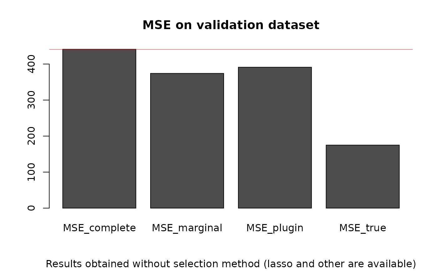
set.seed(1)
# dataset generation
base <- mixture_generator(n = 15, p = 10, ratio = 0.4, tp1 = 1, tp2 = 1, tp3 = 1,
                          positive = 0.5, R2Y = 0.8, R2 = 0.9, scale = TRUE, 
                          max_compl = 3, lambda = 1)

X_appr <- base$X_appr # learning sample
Y_appr <- base$Y_appr # response variable for the learning sample
Y_test <- base$Y_test # responsee variable for the validation sample
X_test <- base$X_test # validation sample
   
TrueZ <- base$Z # True generative structure (binary adjacency matrix)
# Z_i,j=1 means that Xj linearly depends on Xi
   
 
# density estimation for the MCMC (with Gaussian Mixtures)
density <- density_estimation(X = X_appr, nbclustmax = 8, detailed = TRUE)
Bic_null_vect <- density$BIC_vect # vector of the BIC found (1 value per covariate)
   
# MCMC to find the structure
res = structureFinder(X = X_appr, verbose = 0, reject = 0, Maxiter = 900, nbini = 20,
                      candidates = -1, Bic_null_vect = Bic_null_vect, star = TRUE, 
                      p1max = 15, clean = TRUE)
hatZ = res$Z_opt # found structure (adjacency matrix)
hatBic = res$bic_opt # associated BIC

# BIC comparison between true and found structure
bicopt_vect = BicZ(X = X_appr, Z = hatZ, Bic_null_vect = Bic_null_vect)
bicopt_true = BicZ(X = X_appr, Z = TrueZ, Bic_null_vect = Bic_null_vect)
sum(bicopt_vect)
#> [1] 259.9427
sum(bicopt_true)
#> [1] 268.9612

# Structure comparison
compZ = compare_struct(trueZ = TrueZ, Zalgo = hatZ) # qualitative comparison

# interpretation of found and true structure ordered by increasing R2
# <NA>line: name of subregressed covariate
readZ(Z = hatZ, crit = "R2", X = X_appr, output = "all", order = 1) 
#> [[1]]
#>                coefs       var
#> 1  0.756688931044162        R2
#> 2               <NA>         4
#> 3  0.859624940069372 intercept
#> 4   -0.1399117868683         2
#> 5 0.0753356912115381         5
#> 6 -0.420585132044892         6
#> 7  0.386889952414899         8
#> 8  0.158399928444675        10
#> 
#> [[2]]
#>                coefs       var
#> 1  0.911860461449336        R2
#> 2               <NA>         1
#> 3   0.91932024337823 intercept
#> 4  0.117452195745483         2
#> 5 -0.253074594237159         5
#> 6  0.140264670180811         8
#> 7  -0.41875113197976        10
#> 
#> [[3]]
#>                coefs       var
#> 1  0.923279184954364        R2
#> 2               <NA>         9
#> 3   0.72615680052669 intercept
#> 4 -0.478981431253879         3
#> 5  -0.13537277411296         5
#> 6  0.466653365456346         8
#> 7 -0.345854851769902        10
#> 
#> [[4]]
#>                 coefs       var
#> 1   0.959993325124032        R2
#> 2                <NA>         7
#> 3  -0.903716709197091 intercept
#> 4   0.252418293426256         2
#> 5  -0.157191523221045         3
#> 6  -0.199826875526643         5
#> 7 -0.0670800344425359         6
#> 
readZ(Z = TrueZ, crit = "R2", X = X_appr, output = "all", order = 1)
#> [[1]]
#>                coefs       var
#> 1  0.714662171588836        R2
#> 2               <NA>         4
#> 3   0.84058604515217 intercept
#> 4 -0.360058365453026         6
#> 5  0.305086409282352         8
#> 6   0.21237655098617        10
#> 
#> [[2]]
#>                coefs       var
#> 1  0.876810338540551        R2
#> 2               <NA>         1
#> 3  0.883968620534446 intercept
#> 4  0.188189202428782         2
#> 5 -0.234780886884954         5
#> 6 -0.372082898411495        10
#> 
#> [[3]]
#>                coefs       var
#> 1  0.890792585053809        R2
#> 2               <NA>         9
#> 3  0.700168743089247 intercept
#> 4 -0.534495903177699         3
#> 5  0.384756709283009         8
#> 6 -0.361609689733513        10
#> 
#> [[4]]
#>                coefs       var
#> 1  0.947197030815705        R2
#> 2               <NA>         7
#> 3 -0.897165694819893 intercept
#> 4  0.253322024128277         2
#> 5 -0.180820187525035         3
#> 6 -0.210790435701806         5
#> 

# Regression coefficients estimation
select = "NULL" # without variable selection (otherwise,  choose "lar" for example)
resY = correg(X = X_appr, Y = Y_appr, Z = hatZ, compl = TRUE, expl = TRUE, pred = TRUE, 
              select = select, K = 10)

# MSE computation
MSE_complete = MSE_loc(Y = Y_test, X = X_test, A = resY$compl$A) # classical model on X
MSE_marginal = MSE_loc(Y = Y_test, X = X_test, A = resY$expl$A) # reduced model without correlations
MSE_plugin = MSE_loc(Y = Y_test, X = X_test, A = resY$pred$A) # plug-in model
MSE_true = MSE_loc(Y = Y_test, X = X_test, A = base$A) # True model
   
   
# MSE comparison
MSE = data.frame(MSE_complete, MSE_marginal, MSE_plugin, MSE_true)
MSE # estimated structure
#>   MSE_complete MSE_marginal MSE_plugin MSE_true
#> 1     441.0069     374.0534    391.176 174.9802
compZ$true_left
#> [1] 4
compZ$false_left
#> [1] 0

barplot(as.matrix(MSE), main = "MSE on validation dataset",  
        sub = "Results obtained without selection method (lasso and other are available)")
abline(h = MSE_complete, col = "red")